MEMM

Given a linear map (i.e., a matrix) \(C \colon \mathbb{R}^n \to \mathbb{R}^m\) and a vector \(b\in \mathbb{R}^m\) which represents our observations, the canonical linear inverse problem is to determine \(x\in \mathbb{R}^n\) such that \(Cx \approx b\). Of course there need not be any vector \(x\) such that \(Cx = b\) (say if \(C\) is not invertible), and if there are multiple \(x\) that satisfy \(Cx \approx b\) it is not clear how we determine which is best. Furthermore, even if \(C\) were invertible, the problem may be ill-conditioned, in the sense that slight perturbations in the data \(C,b\) may cause the solution \(x\) to vary drastically. These situations are all undesirable, and we say the problem is ill-posed.

A standard approach to determine a solution \(x\) is to frame this as an optimization problem:

Here \(R\) is a regularizer intended to encourage solutions with desirable structure, and \(F(Cx,b)\) is a fidelity term that measures the difference between \(Cx\) and \(b\). It turns out that many popular choices of regularizer and fidelity term can be motivated from a statistical perspective. For example, the Tikhonov regularizer \(R = \|\cdot\|_2^2\) corresponds to performing maximum a posteriori (MAP) estimation with a Gaussian prior assumption on the data. Another example, the \(\ell_1\) regularizer \(R = \|\cdot\|_1\) corresponds to MAP estimation with a Laplacian prior assumption.

It is natural to wonder if there is a meaningful way to choose your regularizer and fidelity terms based on knowledge of the given problem. One answer to this question comes from information theory. In 1957, E.T. Jaynes gave us the Principle of Maximum Entropy, which roughly says that the probability distribution that best represents an unknown model is that with maximum entropy, subject to prior constraints. Taking this a step further, the Principle of Maximum Entropy on the Mean says that the state best describing an unknown system is the mean of the aforementioned maximum entropy distribution.

We can translate these ideas to mathematics by adopting the Kullback-Leibler (KL) divergence as a measure of “distance” between probability distributions:

The expression being integrated is the logarithm of the Radon-Nikodym derivative (when it exists). Now given a probability distribution \(P\) the Maximum Entropy on the Mean (MEM) Function [Rietsch, 1977] \(\kappa_P \colon \mathbb{R}^d \to(-\infty,+\infty]\) is defined by

Despite all this talk of maximizing entropy, we observe that the MEM function is defined by a minimization problem. It can be shown that maximizing entropy is equivalent to minimizing distance from the uniform distribution, so here we are minimizing distance from the prior distribution \(P\) in order to maximize entropy while respecting the prior constraints. Intuitively, the MEM function gives us a way to numerically quantify the compliance of \(y\) with our prior distribution \(P\) by finding the closest distance (in the sense of KL) to a distribution \(Q \ll P\) with mean \(y\). In general the optimization problem defining \(\kappa_P(y)\) is an infinite-dimensional problem over a space of probability measures, so this representation is computationally intractable. We will deal with this shortly.

To be concrete, we can consider reformulating the least squares inverse problem in terms of the MEM paradigm as follows. The solution \(\bar{x}\) is taken as the mean of the distribution minimizing the KL-regularized problem:

We can instead package away all the infinite-dimensionality into the MEM function and write the equivalent problem:

This representation is not of much use unless we understand \(\kappa_P\). Fortunately, our main theoretical result establishes verifiable conditions under which \(\kappa_P\) admits an alternative finite-dimensional characterization as the convex conjugate of a familiar function. To be precise:

Theorem 1 [Vaisbourd et al.]: Suppose \(P \in \mathcal{P}(\Omega)\) generates a minimal and steep exponential family, and that one of the following holds:

• \(\Omega_P \text{ (the support of \(P\)) is uncountable}\)
• \(\Omega_P \text{ is countable and } \mathrm{conv}\Omega_P \text{ is closed}\)

Then \(\kappa_P(y) = \psi_P^*(y) := \sup\{\langle y,\theta - \psi_P(\theta)\}\) where \(\psi_P(\theta) = \log \int_\Omega \exp(\langle y,\theta \rangle) dP(y)\) is the log-moment-generating-function for \(P\).

The minimal and steep exponential family assumption deserves some more attention. The standard exponential family generated by \(P\) is the set of densities

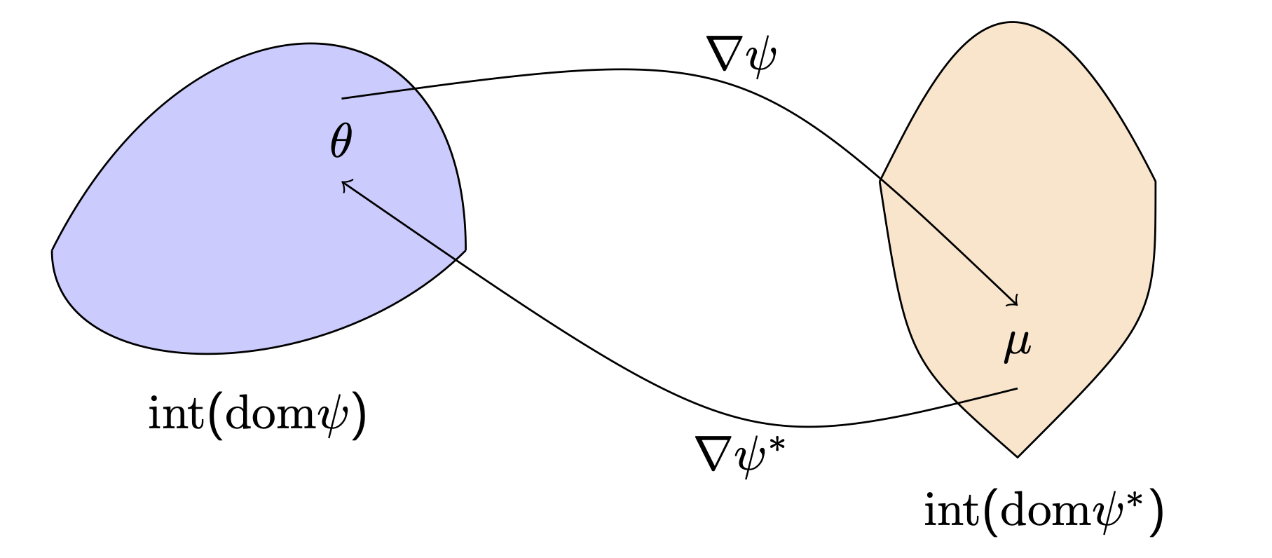
Minimality is a mild topological assumptions on the domain of \(\psi_P\) and steepness is an assumption on the convexity and smoothness of \(\psi_P\). Under these assumptions we have a homeomorphic relationship between the domains of \(\psi_P\) and \(\psi_P^*\):

Now the bulk of the work is to compute these functions \(\psi_P^*\) (known as Cramér’s function from large deviations theory). Fortunately, we have derived closed-form expressions for the Cramér function for many popular probability distributions, as well as their (Bregman) proximal operators for solving the regularized problems algorithmically. For more information, check out our recent preprint, soon to be paired with a Python package allowing users to experiment with solving custom regularized problems in the MEM framework.